It’s been a while since I’ve last made a post. A few things have happened since. One of the big ones is that I got the opportunity to attend the Recurse Center at the beginning of this year. I plan on writing a separate post on my experience.
Today, I wanted to talk about one of the things I’ve continued to be a part of since my batch ended. During my batch, I somehow found myself a part of the quantum computing study group started by Ryan Prior. In the study group, we have been working through the Quantum Country essays by Andy Matuschak and Michael Nielsen. The essays are intended to be a gentle introduction to the field.
I joined the group with zero knowledge of how quantum computers worked, so it has been quite a surprise to learn how much of a central role math plays! As we work through the essays, some of our goals are to document our findings (through an Observable notebook), create interactive visualizations that help with building intuition on the concepts presented, and to have a working quantum computer simulator at the end.
One of the tangible things we have made so far, is an interactive way to visualize the state of a qubit. The first essay in the series states:
The quantum state of a qubit is a vector of unit length in a two-dimensional complex vector space
And presents the following image to illustrate this:
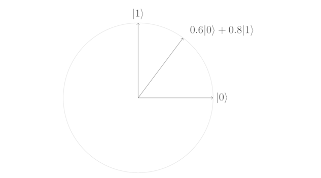
What if this diagram was interactive? Below is a realization of this wish! You can use your mouse to interact with the diagram. (Note, this works best on a wide screen e.g. landscape mode on mobile).
The visuals above only show the real vector space. To quote the essay:
I’ve been talking about quantum states as two-dimensional vectors. What I didn’t yet mention is that in general they’re complex vectors, that is, they can have complex numbers as entries.
…
Because quantum states are in general vectors with complex entries, the illustration above shouldn’t be taken too literally – the plane is a real vector space, not a complex vector space. Still, visualizing it as a plane is sometimes a handy way of thinking.
The typical approach taken to visualize the complex vector space, is to go 3D and use Bloch spheres. Ryan came up with a brilliant idea of how to stay in the 2D world, and build upon the unit circle approach!*
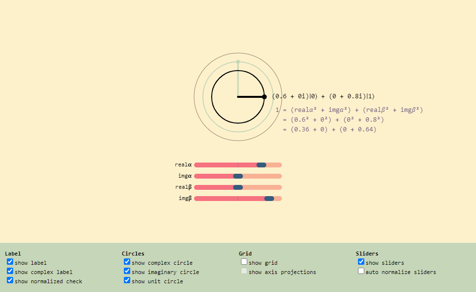
In the earlier visuals, one can say that the circle represents the real component. What if a second circle is added to represent the imaginary component? Below is an interactive visualization of this idea.
The radius of the real circle (black) represents the magnitude of the real component, and the radius of the imaginary circle (green) represents the magnitude of the imaginary component. The state represented is a valid quantum state if the sum of the squares of both magnitudes is equal to one.
As before, you can use your mouse to play with the visualization.
These and other visualizations are some of the things that will be a part of the Observable notebook mentioned earlier. The notebook is currently a work in progress. I will update this post with a link to the notebook once published.
The code for these visualizations can be found on Github.
* The approach is inspired by one of the ways four-dimensional (4D) shapes are visualized in three-dimensional (3D) space. Specifically, Ryan explained how you can visualize these 4D shapes in 3D space by the shadows they cast. (I won’t pretend I understood that, but here is a link to the relevant Wikipedia article).